Manual for the MicroCT
Details
The MicroCT at the departement of clinical research is a Scanco µ40 desktop microtomography system. This wiki-page is a manual for using it and performing measurements on it. If you click on the symbol on the top right besides the title, you can download this page as an OpenOffice-file.
If you have special problems with the machine1) which cannot be solved with this manual, then you can either ask David, or either call or email Mark Siegrist, which is the responsible lab technician for the Scanco MicroCT.
Login
The openVMS-Machine should be running all the time. We login with the username “anatomie” and the password which is either known by David or Sébastien.
<note> Other institutes login with
- bonebiology for the DKF
- mem for the Artorg Center, which used to be the MEMCenter
- microct for external Users
</note>
After login you should see a DECterm (terminal) window, a Session-Manager window and the MicroCT-window on your screen. If you don't see the MicroCT window, it can be started using the “Applications”-Menu in the Session-Manager.
These usernames are also used for remote-access, be it either via ssh or via the web-interface. The web-interface can be accessed with the addition of your username to the host-name of the machine, like ~anatomie for our group, and also need authentification with username/password.
Setup
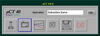
At first, you have to enter your operator name into the MicroCT-Window on the bottom left of the screen (see figure below)
The Operator-numbers are
- Customer/Research Institute, which is a general user
- SCANCO Medical AG, only used for maintenance
- David Haberthür
- Johannes Schittny
- Sonja Mund
- Mohammed Ouanella
- Sebastien Barre
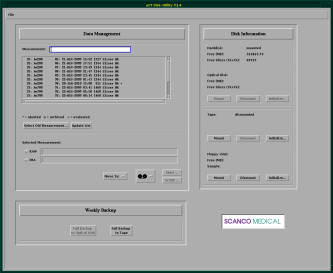
The image above shows the general screen of the MicroCT, where you can start all the necessary programs. The first button opens the sample-definition window, which is generally the first window to open. The second button opens the scanning program, the third button the evaluation program, the fourth the visualization program, the fifth is for the backup-utility and the last is labeled exit because it ends the program.
LogFile
To have a good overview over what you're scanning it's probably best to have some kind of Logfile in your Labbook. You can download a template either as pdf2) or as Microsoft Excel file.
Scan
The quick way:
- Click through all the button from left to right
A thorough explanation of each point can be found below
Define Samples
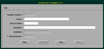
Before you can actually scan a sample, you need to define its properties. For this, you can use the leftmost button on the µCT panel. After starting it, you see the Sampledefinition-Program below.
Press “New” to define a new sample and enter its details in the appropriate fields. Note that each sample gets an unique number. Afterwards, each measurement of the sample also gets an unique number. This makes it possible to search for the all the data for each sample and measurement under DISK2:[ANATOMIE.DATA.Samplenumber.Measurementnumber] (see also the details for remote access).
Start Scan
controlfile
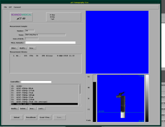
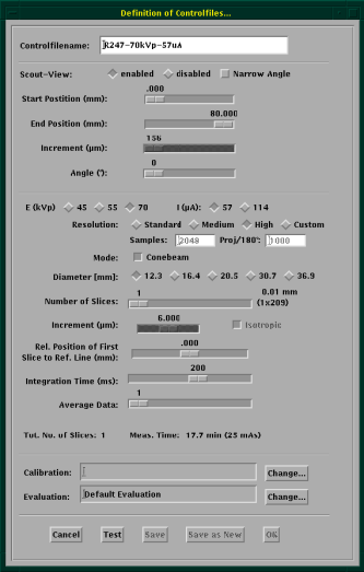
The scanning process at the µCT is controlled and defined by socalled controlfiles. When you start the tomography-program (second button on the start panel), you should get the screen shown below.
First, you need to select, which sample you want to to scan and enter its number (you did write it down before, did you?)
After you have selected the correct sample, select an appropriate controlfile. There are already a bunch of controlfiles set up for our account. Depending on the sample, embedding and staining, you need to choose the appropriate file.
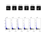
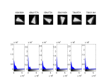
For paraffin embedded rat lung samples we were able to show through empirical observation, that a voltage of 45 kV and a current of 177 mA is suited best. The images below show all the possible configurations for voltage and current. They have been made with this MATLAB script3).
If we look at the histograms on the left we don't see too much difference, but in the normalized histograms on the right, we see that a increase in current shows better “selectability” in the histogram. As a rule of thumb: Use low voltage and high current.
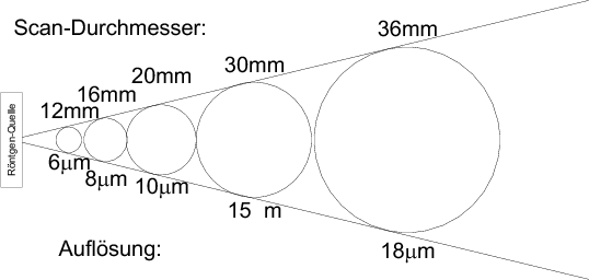
One important thing to note in the controlfile dialog is the diameter of the tube, you've packed your sample into. The diameter of the tube directly influences the field of view and thus the resolution of the scan, see the approximate situation in the fanbeam image below.
Setting the averaging to a higher level increases the scanning time, but can improve the Signal to Noise ration, so use at it depending on your needs. But generally it's better to increase the integration time before averaging several projections.
<note tip>Max out integration time before resorting to frame averaging!</note>
Scout-View
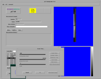
To actually perform the scan, you first have to define the region to scan. This is done with a press of the “Scout-View” button in the Tomography program. Then you must start a Scout-View with the appropriate button. If you would have defined default values for the scanning position in the controlfile, you could just use this button, but since we generally don't have such a prospective study design, we are using a different Scout-View for each sample.
Press the “Scout-View” button and wait (a long time) until the µCT presents you with an overview of the situation in the tube (upper right blue square in the image below). After you see the whole region you want to scan, you can “Cancel” the scout view. Using the “Reference-Line” button, you can mark the region to scan. Use the mouse to position the top of the region at the desired place, use “Shift”+the left mouse button to set the region to the desired height. Watch out for the time (in green) your scan will take. <note tip> Sometimes it's better to scan a bit less slices and have a scan that takes an hour less to perform. Keep an eye on the green text which tells you how long the scan will take. </note>
Perform (Batch) Scan
After you've set the reference line according to your needs, you can either press “OK” and then perform the scan with the “Scan” button in the tomography window, or—if you want to scan multiple samples in one session—you press the “Batch Measurement” button. This adds your currently defined scan to a queue and permits to setup multiple other samples and/or regions for scanning.
Press “Batch Measurement” and your scan will be added to the queue. After you have set up the last scan of your batch measurement, don't add it to the batch with “Batch Measurement”, but press “Start Batch Scans” to start all scans you've set up. Only press the “Start Batch Scan” button once, it takes a long time until the µCT reacts and actually starts the batch scan. When it has started the scan, you can follow the progress of the whole batch with entering
$ que
in the Terminal. Alternatively, you can access the Web Interface and look at the Batch Queues.
<note warning> If you perform a batch scan, double- and triplecheck that you've entered the correct sample number, the correct controlfile and the correct reference line before pressing “Batch Measurement”. If you screwed something up, you can use the
$ que
command to find you the process ID of the wrong scan and then use
$ delete/entry=PID
to delete this scan. </note>
Evaluation
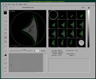
The third button on the µCT-panel starts the Evaluation program. This program is used to evaluate the scanned samples directly on the MicroCT or if you want to export the scanned to a stack of tiff-Files4).
After starting the evaluation program, you need to load a sample that has finished scanning. After the sample has finished loading, you can start drawing a contour on your images. For this, choose the top button on the button bar on the left. Then you can draw a counter-clockwise circle around the sample on some slices.
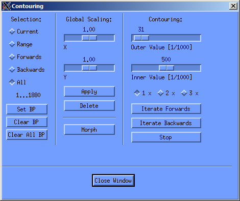
I generally draw a contour on all slices visible in the right cand column, these are aroung 12-16 slices, then doubleclick on the first contour, and let the contouring window open, as seen below. In this window I then click on “All” under selection an let the evaluation program morgph all the missing contours with the “morph” button in the central column. This morphs all contours between the ones I've drawn. If you've got a twitchy hand, you can easily correct the drawn contours. You just need to keep in mind to always draw counterclockwise. If you start the correction inside the already drawn contour, stuff get's added, if you start outside, stuff gets deleted (as seen in the screencast below).
Then in a second step I look at the morphed contours it they're correct, change them if necessary and repeat the morphing step. A quick rundown on the contouring step is shown in the screencast below, including the correction of contours.
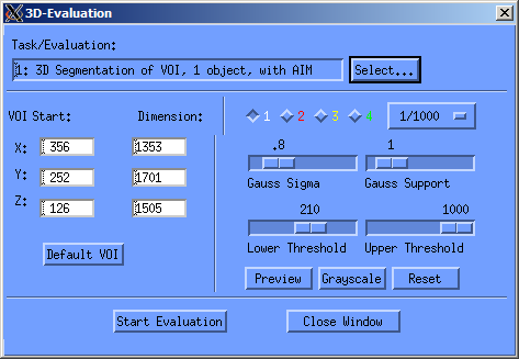
After you've added the contours, you can start the so called evaluation of the sample. To do this, press the lowest button on the sidebar (the one with “T…” on it). If you'd like to work with the 3D visualization program of SCANCO, then you should select Task 1 in the “Task/Evaluation” window, as shown below. Then you only need to choose the correct threshold5). When you press “Start Evaluation”, your sample is evaluated and prepared for three-dimensional analysis, as described in the next section. If you'd like to work with another program for the visualization of your sample, you can choose the figth Evaluation script (Convert to TIFF), and the ISQ-file will be converted to a stack of tiff files which you can then copy from the machine.
Three-dimensional visualization
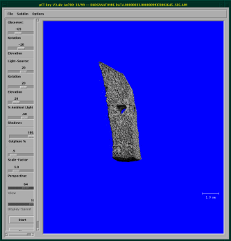
After the evaluation of your sample has finished, you can load them into the evaluation software, the fourth button from the left. Again, as in the evaluation software, you first need to load your sample from disk and can then visualize it in three dimensions. Sophisticated animations can also be made, including cutplane animations.
After you've loaded the sample, the visualization package draws a rough approximation of the sample to the screen and iteratively improves it over time. At any time during drawing, you can stop the process and click into the drawing area. Then you can move and rotate the sample using the mouse. Whenever you let go of the mouse button, the screen is redrawn.
